How to hide rows in Google Sheets

Created by Athan Romblon, Modified on Fri, 2 Feb, 2024 at 5:00 AM by Athan Romblon

Here's the easiest way to hide rows in Google Sheets.

Open a Google Sheets spreadsheet.
Select the rows you want to hide.
Right-click your selection, and click Hide rows [row numbers]. Or, use the keyboard shortcut: command+option+9 on Mac or Ctrl+Alt+9 on Windows.

That's it. A pair of arrows will appear on the rows above and below your hidden selection to indicate there are hidden rows.

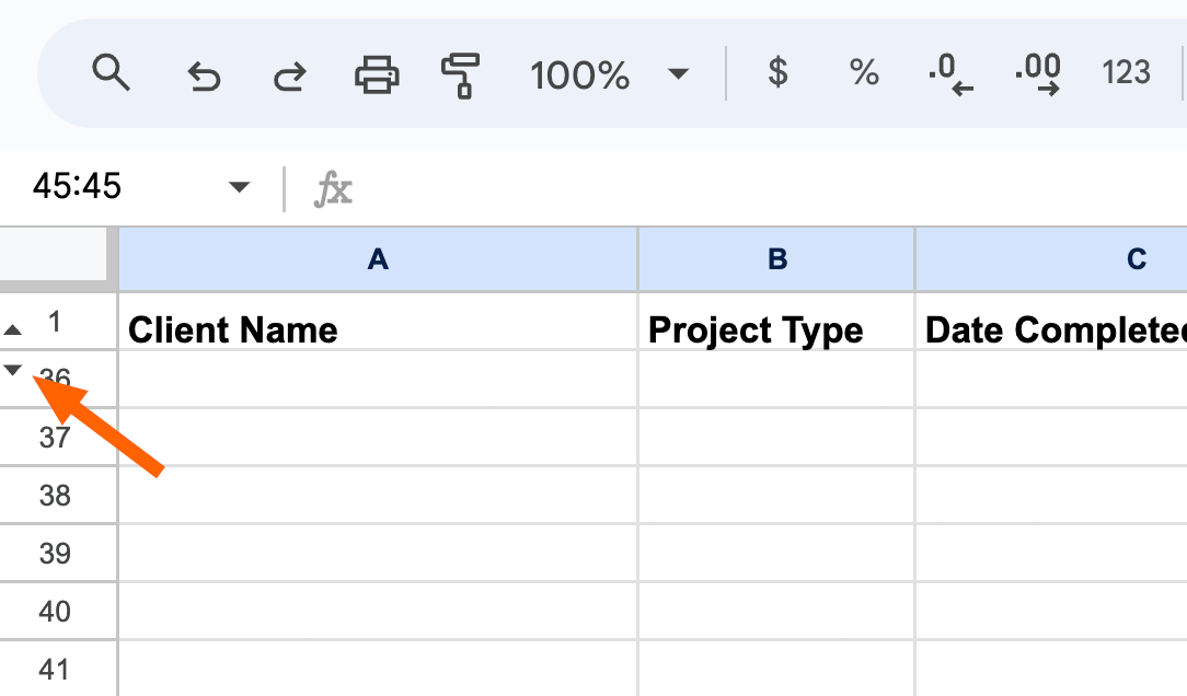
Example of hidden rows in Google Sheets.

To unhide your selection of hidden rows, click the pair of arrows. Alternatively, select the rows above and below your hidden selection, and use your keyboard shortcut: command+shift+9 on Mac or Ctrl+Shift+9 on Windows.

Demo of how to unhide rows in Google Sheets.

Need to hide columns in Google Sheets instead? Select the columns you want to hide, right-click the selection, and click Hide columns [column letters]. The same pair of arrows will appear in the letter header on either side of your hidden selection. Click the arrows to unhide your columns.